Chapter 1: Introduction to the ADAM Algorithm

The ADAM optimization algorithm has gained immense popularity in the realm of machine learning, primarily due to its effectiveness and reliability. This algorithm merges concepts from two other well-known optimization strategies: AdaGrad and RMSprop.

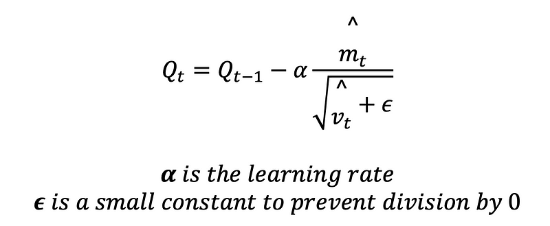
To begin, let’s delve into the equation that defines ADAM and see how it relates to the algorithms we have previously discussed:

If you have been following my earlier posts, you might notice that this equation shares similarities with previous algorithms, particularly with the introduction of the terms ^mt and ^vt. These represent the first-moment estimate (^mt) and the second-moment estimate (^vt).

Chapter 2: Bias-Correction in Moment Estimates

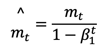
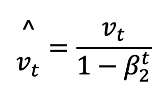
Both the first and second-moment estimates tend to be biased towards zero, especially during the early phases of the optimization when t is small. To remedy this, ADAM employs bias-corrected estimates that accurately reflect the true values:

Bias-corrected first moment:

Bias-corrected second moment:

Now, let's summarize the reasons behind ADAM's prevalence in machine learning. By utilizing both the first and second-moment estimates, ADAM can individually adapt the learning rates for each parameter. Parameters with larger gradients experience a reduction in their learning rates, while those with smaller gradients see an increase. This adaptability significantly enhances convergence speed and overall performance.

The first-moment estimate, representing the mean of the gradients, effectively reduces noise and variance in updates, leading to a more stable convergence. Meanwhile, the second-moment estimate ensures that updates remain manageable, preventing overshooting of the minimum.

Chapter 3: Code Example of ADAM in Action

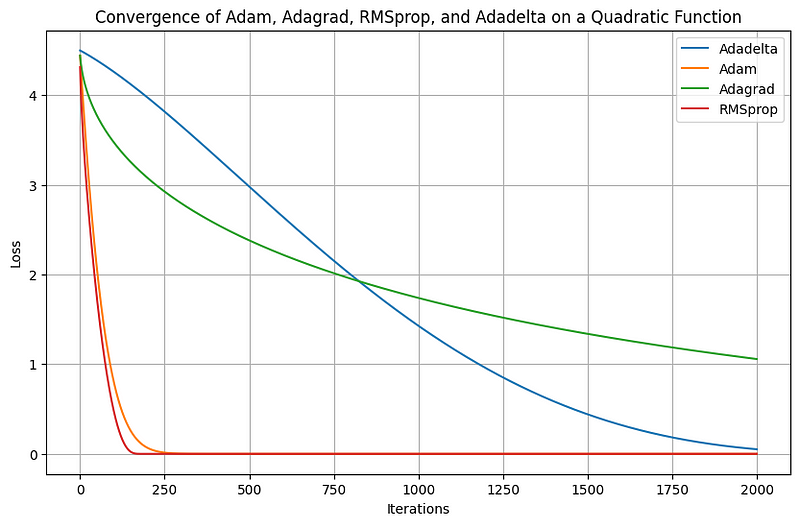
Now, let's take a look at a code example to understand how ADAM stacks up against previously studied algorithms:

import numpy as np

import matplotlib.pyplot as plt

# Define the quadratic function

def quadratic(x, y):

return x**2 + y**2

# Gradient of the quadratic function

def quadratic_grad(x, y):

dfdx = 2 * x

dfdy = 2 * y

return np.array([dfdx, dfdy])

# Number of iterations

iterations = 2000

# Learning rates

learning_rate = 0.01

# AdaDelta parameters

x_adadelta = np.array([1.5, 1.5])

grad_squared_avg_adadelta = np.zeros_like(x_adadelta)

delta_x_squared_avg = np.zeros_like(x_adadelta)

adadelta_loss = []

decay_rate = 0.9

# Adam parameters

x_adam = np.array([1.5, 1.5])

m_adam = np.zeros_like(x_adam)

v_adam = np.zeros_like(x_adam)

beta1 = 0.9

beta2 = 0.999

epsilon = 1e-8

adam_loss = []

# Adagrad parameters

x_adagrad = np.array([1.5, 1.5])

grad_squared_sum_adagrad = np.zeros_like(x_adagrad)

adagrad_loss = []

# RMSprop parameters

x_rmsprop = np.array([1.5, 1.5])

grad_squared_avg_rmsprop = np.zeros_like(x_rmsprop)

rmsprop_loss = []

# Training loop for AdaDelta

for i in range(iterations):

grad = quadratic_grad(x_adadelta[0], x_adadelta[1])

grad_squared_avg_adadelta = decay_rate * grad_squared_avg_adadelta + (1 - decay_rate) * grad**2

delta_x = - (np.sqrt(delta_x_squared_avg + epsilon) / (np.sqrt(grad_squared_avg_adadelta) + epsilon)) * grad

x_adadelta += delta_x

delta_x_squared_avg = decay_rate * delta_x_squared_avg + (1 - decay_rate) * delta_x**2

adadelta_loss.append(quadratic(x_adadelta[0], x_adadelta[1]))

# Training loop for Adam

for t in range(1, iterations + 1):

grad = quadratic_grad(x_adam[0], x_adam[1])

m_adam = beta1 * m_adam + (1 - beta1) * grad

v_adam = beta2 * v_adam + (1 - beta2) * (grad ** 2)

m_hat = m_adam / (1 - beta1 ** t)

v_hat = v_adam / (1 - beta2 ** t)

x_adam -= learning_rate * m_hat / (np.sqrt(v_hat) + epsilon)

adam_loss.append(quadratic(x_adam[0], x_adam[1]))

# Training loop for Adagrad

for i in range(iterations):

grad = quadratic_grad(x_adagrad[0], x_adagrad[1])

grad_squared_sum_adagrad += grad**2

x_adagrad -= (learning_rate / (np.sqrt(grad_squared_sum_adagrad) + epsilon)) * grad

adagrad_loss.append(quadratic(x_adagrad[0], x_adagrad[1]))

# Training loop for RMSprop

for i in range(iterations):

grad = quadratic_grad(x_rmsprop[0], x_rmsprop[1])

grad_squared_avg_rmsprop = decay_rate * grad_squared_avg_rmsprop + (1 - decay_rate) * grad**2

x_rmsprop -= (learning_rate / (np.sqrt(grad_squared_avg_rmsprop) + epsilon)) * grad

rmsprop_loss.append(quadratic(x_rmsprop[0], x_rmsprop[1]))

# Plotting the loss over iterations

plt.figure(figsize=(10, 6))

plt.plot(adadelta_loss, label='Adadelta')

plt.plot(adam_loss, label='Adam')

plt.plot(adagrad_loss, label='Adagrad')

plt.plot(rmsprop_loss, label='RMSprop')

plt.xlabel('Iterations')

plt.ylabel('Loss')

plt.title('Convergence of Adam, Adagrad, RMSprop, and Adadelta on a Quadratic Function')

plt.legend()

plt.grid(True)

plt.show()

In conclusion, the first and second-moment estimates in ADAM play a critical role in providing adaptive learning rates and stabilizing the optimization process. This capability enables ADAM to efficiently tackle various challenges, making it a favored choice for training sophisticated machine learning models.

Thank you for reading! Be sure to subscribe for updates on my future publications. If you found this article valuable, consider following me to stay informed about new posts. For those interested in a deeper exploration of this topic, I recommend my book “Data-Driven Decisions: A Practical Introduction to Machine Learning,” which provides comprehensive insights into starting your journey in machine learning. It’s an affordable investment, akin to buying a coffee, and supports my work!

The first video titled "Adam Optimizer or Adaptive Moment Estimation Optimizer" provides an overview of how the ADAM algorithm functions and its advantages in optimization.

The second video, "ADAM (Adaptive Moment Estimation) Made Easy," simplifies the concepts behind the ADAM algorithm, making it accessible for beginners and enthusiasts alike.