Chapter 1: Introduction to Categorical Variables

A categorical variable is fundamentally designed to categorize or label data. Examples include major global cities, the four seasons of the year, or industry types such as oil, travel, and technology. These variables have a finite number of categories in real-world datasets. Although they can be numerically represented, unlike continuous variables, the values of categorical variables do not possess a meaningful order. For instance, the oil industry is neither superior nor inferior to the travel industry; hence, they are classified as nonordinal.

To determine if a variable should be categorical, consider this question: "Is the distinction between two values significant, or is the mere difference enough?" For example, a stock price of $500 is indeed five times greater than a price of $100, indicating that stock prices should be depicted as continuous numeric variables. Conversely, a company’s industry classification (like oil, travel, or tech) should be treated categorically. Large categorical variables are notably prevalent in transactional data. Many online services, for instance, track users via unique IDs, which can range from hundreds to millions depending on the user base.

IP addresses associated with internet transactions also exemplify large categorical variables. While these identifiers are numeric, their magnitude is not essential for the analysis at hand. For example, during fraud detection, certain IP addresses or subnets may show higher levels of fraudulent activity. However, the numeric value itself (e.g., whether 164.203.x.x is greater than 164.202.x.x) is irrelevant.

The vocabulary of a document corpus can also be viewed as a vast categorical variable, where each unique word represents a category. Representing numerous distinct categories can be computationally intensive. In cases where a category (like a word) appears multiple times in a document, it can be quantified through counts, leading us to a method known as bin counting. This discussion will begin with common ways to represent categorical variables and gradually lead to an exploration of bin counting, particularly relevant for large categorical variables in modern datasets.

Chapter 2: Encoding Categorical Variables

Categorical variables typically consist of non-numeric categories, such as colors (e.g., "black," "blue," "brown"). Therefore, a method for encoding these categories into numeric values is necessary. A straightforward approach might involve assigning integers from 1 to k for each of the k categories; however, this creates a situation where the values could be ordered, which is not appropriate for categorical variables.

One effective encoding technique is one-hot encoding. In this method, each category is represented by a bit. If a variable cannot belong to multiple categories simultaneously, only one bit in the set will be "on." This technique is implemented in scikit-learn as sklearn.preprocessing.OneHotEncoder. Consequently, a categorical variable with k possible categories is transformed into a feature vector of length k.

One-hot encoding is relatively easy to grasp, but it does consume one extra bit than necessary. If k–1 bits are set to 0, the remaining bit must be 1, as the variable must take one of the k values. This constraint can be expressed mathematically as follows:

e1 + e2 + … + ek = 1

Thus, this results in a linear dependency, complicating the interpretation of linear models since various combinations of features can yield identical predictions.

Another approach is dummy coding, which addresses the excess degree of freedom inherent in one-hot encoding. Dummy coding utilizes only k–1 features for representation, effectively discarding one feature and using a vector of all zeros for it, known as the reference category. Both dummy coding and one-hot encoding can be executed in Pandas using pandas.get_dummies.

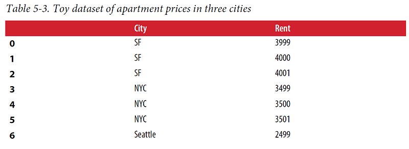
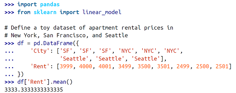
Models utilizing dummy coding tend to be more interpretable than those using one-hot encoding. This becomes evident in a simple linear regression scenario. For example, if we examine rental prices in cities like San Francisco, New York, and Seattle, we can train a linear regression model to predict prices based on city identity.

The linear regression equation can be represented as:

y = w1x1 + … + wnxn

An additional constant term, known as the intercept, is often included so that y can take a non-zero value when all x’s are zero:

y = w1x1 + … + wnxn + b

Example 5–1 illustrates linear regression on a categorical variable using both one-hot and dummy codes:

In Plain English?

Thank you for being a part of the In Plain English community! Before you go, be sure to clap and follow the writer!

Follow us: X | LinkedIn | YouTube | Discord | Newsletter

Visit our other platforms: Stackademic | CoFeed | Venture | Cubed

More content at PlainEnglish.io